Request for help making better dynamic tick marks while zooming

[roland]

I have made four example graphs in the code below. The first three illustrate the sort of tick marks and labels I would like to have. In words, something like when showing multiple years, label with the year in the middle of the year with tick marks on the year boundary, when showing a range less than, say, two years put the ticks on the month boundary and show the month name in the middle of the month, when showing 90 days, use each midnight as the tick and label in the middle as shown. This is all accomplished by setting the tick0, dtick and tickformat according to the initial range of the time axis. But these plots won’t zoom well because the dtick and tickformat won’t change as the plot is zoomed.

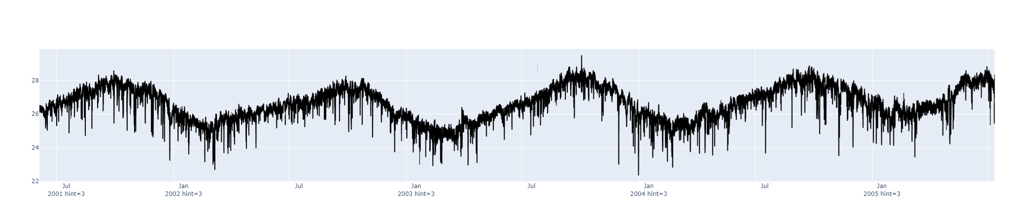
Then last two are examples of the behavior when attempting to using the tickformatstops to get the text of the label as desired when zooming to say nothing of the location of the label or placement of the tickmarks.

Is there a way to achieve the control I want over the ticks with configuration? Or maybe do I have to listen to a callback on the zoom range and make adjustments to tick0, dtick and tickformat after each zoom change?

import datetime

import dash
from dash import Dash, callback, html, dcc, dash_table, Input, Output, State, MATCH, ALL
import pandas as pd
import plotly.graph_objects as go
from plotly.subplots import make_subplots

url_years = 'https://data.pmel.noaa.gov/generic/erddap/tabledap/NTAS_flux.csv?TA_H,time,latitude,longitude,wmo_platform_code&orderByClosest(%22time/48hours%22)&time>=2001-03-31&time<=2004-06-12&wmo_platform_code="48401.0"&depth=5.7'
url_months = 'https://data.pmel.noaa.gov/generic/erddap/tabledap/NTAS_flux.csv?TA_H,time,latitude,longitude,wmo_platform_code&orderByClosest(%22time/24hours%22)&time>=2011-09-25&time<=2012-03-12&wmo_platform_code="48401.0"&depth=5.7'
url_days = 'https://data.pmel.noaa.gov/generic/erddap/tabledap/NTAS_flux.csv?TA_H,time,latitude,longitude,wmo_platform_code&orderByClosest(%22time/3hours%22)&time>=2009-06-04&time<=2009-07-12&wmo_platform_code="48401.0"&depth=5.7'
url_year_to_days = 'https://data.pmel.noaa.gov/generic/erddap/tabledap/NTAS_flux.csv?TA_H,time,latitude,longitude,wmo_platform_code&orderByClosest(%22time/3hours%22)&time>=2001-06-04&time<=2005-07-12&wmo_platform_code="48401.0"&depth=5.7'
app = dash.Dash(__name__)

one_day = 24*60*60*1000
a_yearish = one_day*365.25
for_year = '%Y'
for_day = '%e\n%b-%Y'
for_mon = "%b\n%Y"

app.layout = html.Div(children=[
    html.H4('Help with Ticks'),
    dcc.Graph(id='year-ticks'),
    dcc.Graph(id='mon-ticks'),
    dcc.Graph(id='day-ticks'),
    dcc.Graph(id='dynamic-ticks'),
    html.Div(id='no-show', style={'display': 'none'})
    ]
)


@app.callback(
    [
        Output('year-ticks', 'figure'),
        Output('mon-ticks', 'figure'),
        Output('day-ticks', 'figure'),
        Output('dynamic-ticks', 'figure')
    ],
    [
        Input('no-show', 'children')
    ]
)
def make_plots(lets_go):
    ydf = pd.read_csv(url_years, skiprows=[1])
    ydf.loc[:, 'text_time'] = ydf['time'].astype(str)
    ydf.loc[:, 'time'] = pd.to_datetime(ydf['time'])
    ydf['text'] = ydf['text_time'] + '<br>' + ydf['TA_H'].astype(str)
    y_start_on_year = datetime.datetime.fromtimestamp(ydf['time'].iloc[0].timestamp()).replace(month=1, day=1, hour=0).isoformat()
    plot1 = go.Figure(go.Scattergl(
        x=ydf['time'],
        y=ydf['TA_H'],
        text=ydf['text'],
        hoverinfo='text',
        connectgaps=False,
        name='TA_H',
        marker={'color': 'black', },
        mode='lines+markers',
        showlegend=False,
    ))
    plot1.update_xaxes({
        'tick0': y_start_on_year,
        'dtick': a_yearish,
        'tickformat': for_year,
        'ticklabelmode': 'period',
        'showticklabels': True,
        'zeroline': True,
    })

    mdf = pd.read_csv(url_months, skiprows=[1])
    mdf.loc[:, 'text_time'] = mdf['time'].astype(str)
    mdf.loc[:, 'time'] = pd.to_datetime(mdf['time'])
    mdf['text'] = mdf['text_time'] + '<br>' + mdf['TA_H'].astype(str)
    m_start_on_year = datetime.datetime.fromtimestamp(mdf['time'].iloc[0].timestamp()).replace(month=1, day=1, hour=0).isoformat()
    plot2 = go.Figure(go.Scattergl(
        x=mdf['time'],
        y=mdf['TA_H'],
        text=mdf['text'],
        hoverinfo='text',
        connectgaps=False,
        name='TA_H',
        marker={'color': 'black', },
        mode='lines+markers',
        showlegend=False,
    ))
    plot2.update_xaxes({
        'tick0': m_start_on_year,
        'dtick': 'M1',
        'tickformat': for_mon,
        'ticklabelmode': 'period',
        'showticklabels': True,
        'zeroline': True,
    })

    ddf = pd.read_csv(url_days, skiprows=[1])
    ddf.loc[:, 'text_time'] = ddf['time'].astype(str)
    ddf.loc[:, 'time'] = pd.to_datetime(ddf['time'])
    ddf['text'] = ddf['text_time'] + '<br>' + ddf['TA_H'].astype(str)
    d_start_on_month = datetime.datetime.fromtimestamp(ddf['time'].iloc[0].timestamp()).replace(day=1, hour=0).isoformat()
    plot3 = go.Figure(go.Scattergl(
        x=ddf['time'],
        y=ddf['TA_H'],
        text=ddf['text'],
        hoverinfo='text',
        connectgaps=False,
        name='TA_H',
        marker={'color': 'black', },
        mode='lines+markers',
        showlegend=False,
    ))
    plot3.update_xaxes({
        'tick0': d_start_on_month,
        'dtick': one_day,
        'tickformat': for_day,
        'ticklabelmode': 'period',
        'showticklabels': True,
        'zeroline': True,
    })

    format_hints = [
        dict(dtickrange=[None, one_day], value="%H:%M\n%e-%b-%Y hint=1"),
        dict(dtickrange=[one_day, one_day*90], value="%e\n%b-%Y hint=2"),
        dict(dtickrange=[one_day*90, one_day*365*2], value="%b\n%Y hint=3"),
        dict(dtickrange=[one_day*365*2, one_day*365*100], value="%Y hint=4"),
    ]

    yddf = pd.read_csv(url_year_to_days, skiprows=[1])
    yddf.loc[:, 'time'] = pd.to_datetime(yddf['time'])
    yddf.loc[:, 'text_time'] = yddf['time'].astype(str)
    yddf['text'] = yddf['text_time'] + '<br>' + yddf['TA_H'].astype(str)
    print('hint3 min= ' + str(one_day*90))
    print('hint3 max=' + str(one_day*365*2))
    interval = yddf['time'].iloc[-1].timestamp()*1000 - yddf['time'].iloc[0].timestamp()*1000
    print('time range in millis=' + str(interval))
    plot4 = go.Figure(go.Scattergl(
        x=yddf['time'],
        y=yddf['TA_H'],
        text=yddf['text'],
        hoverinfo='text',
        connectgaps=False,
        name='TA_H',
        marker={'color': 'black', },
        mode='lines',
        showlegend=False,
    ))
    plot4.update_xaxes({
        'tickformatstops': format_hints,
        'ticklabelmode': 'period',
        'showticklabels': True,
        'zeroline': True,
    })

    return [plot1, plot2, plot3, plot4]


if __name__ == '__main__':
    app.run_server(debug=True)

[roland]

I’m going to answer my own question for folks who happen along later:

It’s pretty straight forward to listen on a callback to the layout changes and set the tick marks. It’s up to you if you want the Loader animation during each resize as I did below. The catch is if you have a long time series (these are hourly data over decades) it’s easy to cause creation of thousands and thousands of tick marks for the graph data structure when you zoom back out before the callback sets new dtick value and this will freeze up while the browser constructs all those tick marks. So through experimentation I came up with some tick refinements that are allowed based on the time range of the entire data set being graphed. In code below you can experiment yourself based on the size of the original data request.

*edited for clarity on why it might be slow zooming back out.

import datetime
import dateutil

import dash
from dash import Dash, callback, html, dcc, dash_table, Input, Output, State, MATCH, ALL
import pandas as pd
import plotly.graph_objects as go

start_date = '2001-04-01'
# decade
end_date = '2010-03-31'
# year
# end_date = '2002-03-31'
# 15 days
# end_date = '2001-04-15'
# 3 days
# end_date = '2001-04-03T23:59'

url_year_to_days = 'https://data.pmel.noaa.gov/generic/erddap/tabledap/NTAS_flux.csv?TA_H,time,latitude,longitude,wmo_platform_code&time>='+start_date+'&time<='+end_date+'&wmo_platform_code="48401.0"&depth=5.7'

app = dash.Dash(__name__)

one_day = 24*60*60*1000
a_yearish = one_day*365.25
for_year = '%Y'
for_day = '%e\n%b-%Y'
for_mon = "%b\n%Y"

df = pd.read_csv(url_year_to_days, skiprows=[1])
df.loc[:, 'time'] = pd.to_datetime(df['time'])
df.loc[:, 'text_time'] = df['time'].astype(str)
df['text'] = df['text_time'] + '<br>' + df['TA_H'].apply(lambda x: '{0:.2f}'.format(x))
time_max = df['time'].iloc[-1].timestamp()
time_min = df['time'].iloc[0].timestamp()
data_range = time_max*1000 - time_min*1000

app.layout = html.Div(children=[
    html.H4('Dynamic Ticks'),
    dcc.Loading(dcc.Graph(id='dynamic-ticks')),
    html.Div(id='no-show', style={'display': 'none'}),
    ]
)


@app.callback(
    [
        Output('dynamic-ticks', 'figure'),
    ],
    [
        Input('no-show', 'children'),
        Input('dynamic-ticks', 'relayoutData')
    ],
    [
        State('dynamic-ticks', 'figure'),
    ]
)
def make_plots(lets_go, relay_data, current_figure):

    if current_figure is not None and relay_data is not None:
        if 'xaxis.range[0]' in relay_data and 'xaxis.range[1]' in relay_data:
            print('zooming in:', datetime.datetime.now().isoformat())
            in_time_min = dateutil.parser.parse(relay_data['xaxis.range[0]'])
            in_time_max = dateutil.parser.parse(relay_data['xaxis.range[1]'])
            ticks = get_ticks(in_time_min.timestamp(), in_time_max.timestamp())
            current_figure['layout']['xaxis']['dtick'] = ticks['dtick']
            current_figure['layout']['xaxis']['tickformat'] = ticks['tickformat']
            current_figure['layout']['xaxis']['tick0'] = ticks['tick0']
            return [current_figure]
        elif 'xaxis.autorange' in relay_data:
            print('resetting zoom to original:', datetime.datetime.now().isoformat())
            ticks = get_ticks(time_min, time_max)
            current_figure['layout']['xaxis']['dtick'] = ticks['dtick']
            current_figure['layout']['xaxis']['tickformat'] = ticks['tickformat']
            current_figure['layout']['xaxis']['tick0'] = ticks['tick0']
            return [current_figure]
        else:
            raise dash.exceptions.PreventUpdate

    ticks = get_ticks(time_min, time_max)

    plot = go.Figure(go.Scattergl(
        x=df['time'],
        y=df['TA_H'],
        text=df['text'],
        hoverinfo='text',
        connectgaps=False,
        name='TA_H',
        marker={'color': 'black', },
        mode='lines',
        showlegend=False,
    ))
    plot.update_xaxes(ticks)
    plot.update_xaxes({
        'ticklabelmode': 'period',
        'showticklabels': True,
        'zeroline': True,
    })

    return [plot]


def get_ticks(time_min, time_max):
    max_ticks = 366
    interval = time_max*1000 - time_min*1000
    if interval <= one_day:
        dtick = 60*60*1000  # one hour
        tick_count = data_range/dtick
        if tick_count > 72:
            dtick=one_day
        dtickformat = "%H:%M\n%e-%b-%Y"
        print('tick_count=', tick_count, 'dtick=', dtick)
        tick0 = datetime.datetime.fromtimestamp(time_min).replace(hour=0, minute=0).isoformat()
    elif one_day < interval <= one_day*45:
        dtick = one_day
        tick_count = data_range/dtick
        if tick_count > max_ticks:
            dtick = "M1"
        dtickformat = "%e\n%b-%Y"
        print('tick_count=', tick_count, 'dtick=', dtick)
        tick0 = datetime.datetime.fromtimestamp(time_min).replace(day=1, hour=0, minute=0).isoformat()
    elif one_day*45 < interval <= one_day*365.0*2:
        dtick = "M1"
        monthish = one_day*30.25
        tick_count = data_range/monthish
        if tick_count > max_ticks:
            dtick = one_day*365
        dtickformat = "%b\n%Y"
        print('tick_count=', tick_count, 'dtick=', dtick)
        tick0 = datetime.datetime.fromtimestamp(time_min).replace(month=1, day=1, hour=0, minute=0).isoformat()
    else:
        dtick = one_day*365.0
        dtickformat = "%Y"
        print('dtick=', dtick)
        tick0 = datetime.datetime.fromtimestamp(time_min).replace(month=1, day=1, hour=0, minute=0).isoformat()
    return {'dtick': dtick, 'tickformat': dtickformat, 'tick0': tick0}


if __name__ == '__main__':
    app.run_server(debug=True)