Hello all,
I am interested in efficiently showing a 3D structure using isocontours. My data is obtained in cylindrical coordinates, with an azimuthal decomposition q(x,r,\theta)=\hat{q}(x,r)e^{im\theta}. It is quite large (about 600k values raw), and I also know a lot about where I expect my surfaces to be spatially.
Right now, I followed the directions at this page : 3d isosurface plots in Python. This leads to a meshgrid to obtain a coarse structured grid of inhomogenous spacing in x, but regular in y and z. I project this Cartesian grid onto the \theta=0 plane, interpolate, then obtain \theta through the function numpy.arctan2. It takes time and it produces very large plots with poor resolution. If I deviate from this process by introducing an inhomogeneous grid, I obtain a blank plot. I increase resolution, I get monsters my navigator cannot handle.
My question is this : if I know that my data is located around r=1 for instance, can I leverage that ? Isocontour is not permissive when it comes to the mesh and its underlying requirements are unclear to me. It seems only capable to handle homogeneous meshes…
To illustrate my point, consider this data in the x-r plane :
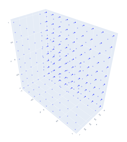
I have to project it on a clearly inadequate mesh that looks something like this (intentionally coarsified for clarity) :
And it gives out something ugly :
Any ideas ?
Hi @hawkspar, I’m not really sure what exactly do you try to plot, maybe a extract of your data and some code which creates the current status of your figures.
In general I would recommend the forum search, specially @empet has a lot of great answers dealing with scientific data and 3d plots in general. Maybe this helps to get some insights concerning the “plotly way” of plotting.
Thanks for the quick answer ! I’m plotting isocontours of modes right now. I have an application that generates my fields (scalars or vectors) in the x-r plane for a prescribed azimuthal wavenumber m. Therefore I am plotting numerical results that are smooth, but do not have an analytical expression. I want to plot these efficiently in 3D.
I’m not sure what you’re asking for - you really think the 600k data would be useful and insightful ? I have already provided an x-r plane view of what a representative function looks like here.
I can give you pseudo-code, which will probably be clearer than a snippet from my application :
1. Compute functions in x-r plane with refined mesh
2. Create a coarse structured cartesian mesh that is homogeneous in y and z, not x
3. Project the cartesian mesh onto the x-r plane, interpolate function onto new mesh
4. Do the azimuthal decomposition - multiply by e^(i m arctan2(Z,Y))
5. If necessary, correct orientation - rewrite e_r and e_theta in cartesian coordinates
6. Use go.Isosurface for 2 surfaces at 10% of min/max of the real part of the function
For 1 see this representative image from the first post, for 2 see a representative mesh and a result is visible here. My current problem is with resolution, file size, and computation speed, in that order.
Google and a forum search did not yield much useful information. I feel like isocontours are much less used than most 3d plotting solutions, which is a shame.


