Hi!
This is my first time posting a question on a forum. Please let me know if my description of the issue is unclear!
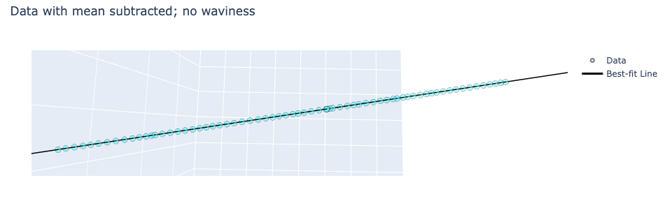
I’m using Plotly to plot a 3D dataset and the best-fit line to that dataset (Plotly version 6.2.0, Mac OS Monterey). When I plot the data in its original coordinates, the dataset and best-fit line appear jagged/wavy/sinuous (see screenshots below). However, if I simply subtract the mean from the dataset and run the exact same plotting functions, the line and dataset appear exactly how I would expect.
My best guess is this has to do with the large values and orders-of-magnitude differences in the x, y, and z dimensions of the dataset. From what I’ve read online, one possible way to smooth the appearance of the line would be to use a “spline” setting for the “line_shape” attribute. However, I would like the best-fit line and data points to appear collinear with their original values and would prefer to avoid interpolating to force smoothness, if possible.
Screenshot of the original dataset, showing waviness:

Screenshot of the same dataset with the mean removed, showing the smoothness I would expect to observe:
The relevant snippet of the original code is below. I’ve included the dataset I’m using and have formatted it exactly as it appears in my original code – apologies for the size of the initial lists!
Thanks to all who respond.
import pandas as pd
import numpy as np
import plotly.graph_objects as go

### Part one: Original dataset ###
# Original dataset
x = [
    242841.51371370474,
    242842.2321057521,
    242842.98216472793,
    242843.7898302282,
    242844.67710247508,
    242845.65306961897,
    242846.62956138235,
    242847.6035021302,
    242848.5577261343,
    242849.4414346082,
    242850.35453927377,
    242851.28328216364,
    242851.98668249528,
    242852.68263891042,
    242853.5190912554,
    242854.48127683587,
    242855.2495724535,
    242855.8670268352,
    242856.67226444918,
    242857.19432551065,
    242858.0543204225,
    242858.91632437005,
    242859.84946477137,
    242860.8340063954,
    242861.76712610642,
    242862.47551305266,
    242863.28264827665,
    242864.24918054775,
    242865.1861166324,
    242865.89921764264,
    242865.96585560686,
    242865.54343995376,
    242866.04327942675,
    242866.95609290188,
    242867.93530624994,
    242868.87682222814,
    242869.6040531725,
    242870.2818274008,
    242871.195308515,
    242872.02078952064,
    242872.80658931847,
    242873.68504109397,
    242874.63072940378,
    242875.61506473337,
    242876.59956580945,
    242877.56710429245,
    242878.4417633086,
    242879.31683372613,
    242880.13168928024,
    242880.92023267024,
    242881.71379591143,
    242882.54724389955,
    242883.4482578614,
    242884.30376656697,
    242885.19765295103,
    242886.11825244414,
    242886.9600141796,
    242887.36266717812,
    242888.00615052023,
    242888.76926449002,
    242889.5641237527,
    242890.47554397324,
    242891.45691368319,
    242892.43368979736,
    242893.4122051768,
    242894.29546648718,
    242895.14065051088,
    242896.09998258963,
    242897.0531311911,
    242897.89569041005,
]
y = [
    3906806.867605061,
    3906806.99149825,
    3906807.120852687,
    3906807.2601418886,
    3906807.413159992,
    3906807.5814743303,
    3906807.749879144,
    3906807.9178440124,
    3906808.08240855,
    3906808.2348120487,
    3906808.392285186,
    3906808.552455276,
    3906808.6737630083,
    3906808.793786971,
    3906808.9380407236,
    3906809.103978307,
    3906809.2364778174,
    3906809.3429633956,
    3906809.4818338864,
    3906809.571868026,
    3906809.720181907,
    3906809.868842264,
    3906810.0297707445,
    3906810.1995638297,
    3906810.3604887417,
    3906810.482656461,
    3906810.6218542117,
    3906810.7885414213,
    3906810.9501245017,
    3906811.073105204,
    3906811.084597522,
    3906811.011748132,
    3906811.0979499584,
    3906811.2553728768,
    3906811.4242470525,
    3906811.5866199764,
    3906811.7120375135,
    3906811.8289257935,
    3906811.9864638527,
    3906812.1288254987,
    3906812.264343763,
    3906812.4158406965,
    3906812.5789331766,
    3906812.7486906843,
    3906812.918476776,
    3906813.0853375164,
    3906813.2361803544,
    3906813.387094142,
    3906813.5276233335,
    3906813.6636147546,
    3906813.8004718944,
    3906813.944207519,
    3906814.099595505,
    3906814.2471356993,
    3906814.40129447,
    3906814.5600601574,
    3906814.7052295627,
    3906814.7746707047,
    3906814.885645212,
    3906815.0172511004,
    3906815.154331751,
    3906815.31151439,
    3906815.48076045,
    3906815.6492143027,
    3906815.8179681073,
    3906815.9702944886,
    3906816.116054098,
    3906816.2814995693,
    3906816.4458786445,
    3906816.591185583,
]
z = [
    663.4151597804555,
    663.4437289572488,
    663.4735574715868,
    663.5056768951674,
    663.540962137783,
    663.5797746190462,
    663.6186079634939,
    663.6573398585826,
    663.6952876537634,
    663.7304311714518,
    663.7667437235136,
    663.8036781800032,
    663.8316511628669,
    663.8593281143825,
    663.89259233969,
    663.9308567526336,
    663.9614105058508,
    663.9859655708151,
    664.0179884416671,
    664.0387498835784,
    664.0729503549891,
    664.1072307221838,
    664.1443400598992,
    664.1834935330202,
    664.2206020479188,
    664.2487733395961,
    664.2808716750297,
    664.3193089481462,
    664.3565692334507,
    664.3849279950878,
    664.3875780686622,
    664.3707793477998,
    664.3906570765743,
    664.4269580485095,
    664.4658996255514,
    664.5033420450945,
    664.5322627291333,
    664.5592166073463,
    664.595544130102,
    664.6283720447158,
    664.6596219081147,
    664.6945563762371,
    664.7321647220051,
    664.7713099911615,
    664.8104618517616,
    664.8489391401395,
    664.883722776953,
    664.9185227744699,
    664.9509281337324,
    664.9822871049239,
    665.0138457066884,
    665.0469904540547,
    665.0828221802874,
    665.1168442432357,
    665.1523925183491,
    665.1890031264005,
    665.2224784967451,
    665.2384912919068,
    665.2640814824322,
    665.2944291707121,
    665.3260393129514,
    665.3622848776236,
    665.4013122093502,
    665.4401568619255,
    665.4790706819934,
    665.5141964167825,
    665.5478078854554,
    665.5859588196997,
    665.6238638480258,
    665.657370932874,
]

# Dataset converted into dictionary and Pandas DataFrame
data_dict = {"x": x, "y": y, "z": z}
test_data = pd.DataFrame(data_dict)

# Calculate mean of dataset
data_mean = [test_data["x"].mean(), test_data["y"].mean(), test_data["z"].mean()]

# Best-fit 3D line to dataset
vector_in = np.array([11.92932516, 2.05731974, 0.47440809])

# Plot best-fit line
linearspacing = np.linspace(-100, 100, 1000)
plot_line_x = data_mean[0] + (vector_in[0] * linearspacing)
plot_line_y = data_mean[1] + (vector_in[1] * linearspacing)
plot_line_z = data_mean[2] + (vector_in[2] * linearspacing)

# Plot of dataset and line - line and dataset appear wavy/jagged
test_figure = go.Figure(
    data=[
        go.Scatter3d(
            x=test_data["x"],
            y=test_data["y"],
            z=test_data["z"],
            name="Data",
            mode="markers",
            marker=dict(
                size=5, line=dict(width=2, color="Black"), color="cyan", opacity=0.5
            ),
        )
    ]
)
test_figure.add_trace(
    go.Scatter3d(
        x=plot_line_x,
        y=plot_line_y,
        z=plot_line_z,
        mode="lines",
        name="Best-fit Line",
        line=dict(color="black", width=3),
    )
)
test_figure.update_layout(
    title="Original data; best-fit line and datapoints appear wavy",
    scene=dict(
        xaxis=dict(range=[data_mean[0] - 40, data_mean[0] + 40]),
        yaxis=dict(range=[data_mean[1] - 40, data_mean[1] + 40]),
        zaxis=dict(range=[data_mean[2] - 40, data_mean[2] + 40]),
    ),
)
test_figure.show()

### Part two: Original dataset with mean subtracted ###
# Same dataset with mean subtracted
x2 = x - data_mean[0]
y2 = y - data_mean[1]
z2 = z - data_mean[2]

# Mean-subtracted dataset converted into dictionary and Pandas DataFrame
data_dict2 = {"x2": x2, "y2": y2, "z2": z2}
test_data2 = pd.DataFrame(data_dict2)

# Same vector plotted, but centered at origin
plot_line_x2 = vector_in[0] * linearspacing
plot_line_y2 = vector_in[1] * linearspacing
plot_line_z2 = vector_in[2] * linearspacing

# Plot of dataset and line
test_figure2 = go.Figure(
    data=[
        go.Scatter3d(
            x=test_data2["x2"],
            y=test_data2["y2"],
            z=test_data2["z2"],
            name="Data",
            mode="markers",
            marker=dict(
                size=5, line=dict(width=2, color="Black"), color="cyan", opacity=0.5
            ),
        )
    ]
)
test_figure2.add_trace(
    go.Scatter3d(
        x=plot_line_x2,
        y=plot_line_y2,
        z=plot_line_z2,
        mode="lines",
        name="Best-fit Line",
        line=dict(color="black", width=3),
    )
)
test_figure2.update_layout(
    title="Data with mean subtracted; no waviness",
    scene=dict(
        xaxis=dict(range=[-40, 40]),
        yaxis=dict(range=[-40, 40]),
        zaxis=dict(range=[-40, 40]),
    ),
)
test_figure2.show()