Figure Friday 2025 - week 38

[adamschroeder]

join the Figure Friday session on September 26, at noon Eastern Time, to showcase your creation and receive feedback from the community.

Which players finished in the top 20 in their respective sport at the end of each season?

Answer this question and a few others by using Plotly on the One-hit wonder dataset.

Things to consider:

• what can you improve in the app or sample figure below (bar chart)?
• would you like to tell a different data story using a Dash app?
• how can you explore the data with Plotly Studio?

Sample figure:

Code for sample figure:

import plotly.express as px
import pandas as pd

df = pd.read_csv("https://raw.githubusercontent.com/plotly/Figure-Friday/refs/heads/main/2025/week-38/one-hit-wonders.csv")

fig = px.bar(df, x='name', y='played_val', hover_data='year', labels={'played_val': 'games played'})
fig.show()

For community members that would like to build the data app with Plotly Studio, simply go to Plotly.com/studio to download and start building.

Below is a screenshot of a bar chart built by Plotly Studio on top of this dataset:

Participation Instructions:

• Create - use the weekly data set to build your own Plotly visualization or Dash app. Or, enhance the sample figure provided in this post, using Plotly or Dash.
• Submit - post your creation to LinkedIn or Twitter with the hashtags #FigureFriday and #plotly by midnight Thursday, your time zone. Please also submit your visualization as a new post in this thread.
• Celebrate - join the Figure Friday sessions to showcase your creation and receive feedback from the community.

If you prefer to collaborate with others on Discord, join the Plotly Discord channel.

Data Source:

Thank you to The Pudding for the data.

[Mike_Purtell]

Here is a dashboard looking at athletic rankings over time. A few points:

• Athletes with fewer than 5 years of data were excluded

• Athletes within each league were first sorted by median rank (to minimize the influence of outliers) across all their years, then by mean rank. The top 5 athletes from each league were selected based on these criteria.

• For the first time I used the Dash Mantine ChipGroup for league selection (allowing single or multiple selections). It was a great learning experience.

• Normally, I turn off all grid lines, but with the y-axis logarithmic (log_y=True), I decided to keep the horizontal grid lines for better clarity.

• It’s been said that athletes from different decades can’t be fairly compared, however this dashboard allows for it. The timeline on the left plots rank by calendar years, while the timeline on the right plots rank by career years. The dataset starts career years at 0, I changed to start at 1.

I have questions about what the ranks truly represent and would love to see a data set like this one covering a far greater number of years.

Here is a link to Plotly Cloud hosted dashboard:

Dash

Here is a screenshot comparing MLB players Mike Trout and Aaron Pujols

Here is the code:

import polars as pl
import plotly.express as px
import dash
from dash import Dash, dcc, html, Input, Output
import dash_mantine_components as dmc

pl.Config().set_tbl_cols(10)

dash._dash_renderer._set_react_version('18.2.0')

'''
    This dashboard has timeline plots of RANK by year and by calendar year. 
    added column RANK_MED is the median rank of each athlete
    added column RANK_MEAN is the mean rank of each athlete
    athletes within each league are ranked by RANK_MED, and then by RANK_MEAN.
    The top 5 athletes are included in this dashboard. Could be ehanced for 
    analysis of lower ranked athletes
'''

viz_template = 'plotly_dark'

#----- LOAD AND CLEAN THE DATASET
df_league_names = pl.DataFrame({
    'LEAGUE_ABBR': ['ATP', 'LPGA', 'MLB', 'NBA', 'NHL', 'PGA', 'WNBA', 'WTA'],
    'LEAGUE_NAME': [
        'Association of Tennis Professionals', 
        'Ladies Professional Golf Association', 
        'Major League Baseball', 
        'National Basketball Association', 
        'National Hockey League', 
        'Professional Golf Association', 
        'Womens National Basketball Association',  
        'Womens Tennis Association'
        ]
})
dict_league_abbr_name = dict(zip(
    df_league_names['LEAGUE_ABBR'], df_league_names['LEAGUE_NAME']))

df  = (
    pl.scan_csv('one-hit-wonders.csv')
    .rename(  # upper case all column names, replace spaces with underscores
        lambda c: 
            c.upper()            # column names to upper case
            .replace(' ', '_')   # blanks replaced with underscores
    )
    .filter(~ pl.col('DNP'))
    .select(
        NAME = pl.col('NAME').str.to_titlecase(),
        FAMILY_NAME = pl.col('NAME').str.to_titlecase().str.split(' ' ).list.last(),
        NAME_COUNT = pl.len().over('NAME').cast(pl.UInt8),
        YEAR = pl.col('YEAR').cast(pl.UInt16),
        YEARS_TOT = pl.col('YEAR').cast(pl.UInt16).len().over('NAME'),
        CAREER_YEAR = (1 + pl.col('YEAR_INDEX')),
        PEAK_CAREER_YEAR = pl.col('PEAK_YEAR_INDEX'),
        TEAM = pl.col('TEAM'),
        PLAYED_VAL = pl.col('PLAYED_VAL').cast(pl.UInt16),
        RANK = pl.col('RANK'),
        RANK_MED = pl.col('RANK').cast(pl.UInt16).median().over('NAME', 'LEAGUE').cast(pl.Float32),
        RANK_MEAN = pl.col('RANK').cast(pl.UInt16).mean().over('NAME').cast(pl.Float32),
        FIRST_YEAR = pl.col('YEAR').min().over('NAME').cast(pl.UInt16),
        LEAGUE_ABBR = pl.col('LEAGUE').str.to_uppercase(),
        NAME_ORG = (  # form of NAME_ORG is NBA: Stephen Curry,  etc.
            pl.col('LEAGUE').str.to_uppercase() + pl.lit(': ') +
            pl.col('NAME').str.to_titlecase()
        )
    )
    .collect()
    .join(df_league_names, on = 'LEAGUE_ABBR', how='left')
)

top_5_list = sorted(list(
    df
    .lazy()
    .unique('NAME_ORG')    
    .sort('LEAGUE_ABBR', 'RANK_MED', 'RANK_MEAN')
    .with_columns(
        RANK_LEAGUE = 
            pl.col('LEAGUE_ABBR')
            .cum_count()
            .over('LEAGUE_ABBR')
            .cast(pl.UInt8)
        )
    .filter(pl.col('RANK_LEAGUE') <= 5)
    .collect()
    ['NAME_ORG']
))

# #----- FUNCTIONS ---------------------------------------------------------------
def get_tl_by_year(df_callback, name_org_list):
    # timeline by calendar year
    fig = px.line(
        df_callback.sort('YEAR'),
        x='YEAR',
        y='RANK',
        color='NAME_ORG',
        template=viz_template,
        markers=True,
        line_shape='spline',
        category_orders={'NAME_ORG': name_org_list}, # handy way to sort legend
        log_y=True,
        title='Timeline by calendar year',
    )
    fig.update_layout(
        xaxis_title='CALENDAR YEAR', yaxis_title='RANK -- LOG SCALE',
        legend_title = 'Athlete'
        )
    fig.update_yaxes(autorange='reversed')
    fig.update_xaxes(showgrid=False)
    return fig

def get_tl_by_career_year(df_callback, name_org_list):
    # timeline by career year
    fig = px.line(
        df_callback.sort('YEAR'),
        x='CAREER_YEAR',
        y='RANK',
        color='NAME_ORG',
        template=viz_template,
        markers=True,
        line_shape='spline',
        category_orders={'NAME_ORG': name_org_list}, # handy way to sort legend
        log_y=True,
        title='Timeline by career year'
    )
    fig.update_layout(
        xaxis_title='CAREER YEAR', yaxis_title='RANK -- LOG SCALE',
        legend_title = 'Athlete'
        )
    fig.update_yaxes(autorange='reversed')
    fig.update_xaxes(showgrid=False)
    return fig

#----- GLOBALS -----------------------------------------------------------------
style_horizontal_thick_line = {'border': 'none', 'height': '4px', 
    'background': 'linear-gradient(to right, #007bff, #ff7b00)', 
    'margin': '10px,', 'fontsize': 32}

style_h2 = {'text-align': 'center', 'font-size': '40px', 
            'fontFamily': 'Arial','font-weight': 'bold', 'color': 'gray'}

#----- DASH COMPONENTS------ ---------------------------------------------------
data = [[i,v] for i, v in dict_league_abbr_name.items()]
dmc_select_league = dmc.Box([
        dmc.Group(
            dmc.ChipGroup(
                [dmc.Chip(k, value=v) for k,v in dict_league_abbr_name.items()],
                multiple=True,
                deselectable=True,
                value=[df_league_names.item(0, 'LEAGUE_NAME')],
                id='select-leagues',
            ),
            justify='left',
        ),
    ])

dmc_selected_leagues = dmc.GridCol(
    dmc.GridCol(
        dmc.Text(
            id='selected_leagues',
            style={'fontSize': '18px','color': 'blue'}
        ), 
    )
)
#----- DASH APPLICATION STRUCTURE---------------------------------------------
app = Dash()
server = app.server
app.layout =  dmc.MantineProvider([
    html.Hr(style=style_horizontal_thick_line),
    dmc.Text(
        'Consistency - top 5 athletes per league', 
        ta='center', 
        style=style_h2
    ),
    html.Hr(style=style_horizontal_thick_line),
    dmc.Grid(children = [dmc.GridCol(dmc_select_league, span=8, offset = 1)]),
    dmc.Grid(children = [
        dmc.GridCol(dmc_selected_leagues, span=8, offset = 1)]),
    dmc.Grid(children = [
        dmc.GridCol(dcc.Graph(id='by-year'), span=6, offset=0),            
        dmc.GridCol(dcc.Graph(id='by-career-year'), span=6, offset=0), 
    ]),
])

@app.callback(
    Output('selected_leagues', 'children'), 
    Output('by-year', 'figure'), 
    Output('by-career-year', 'figure'), 
    Input('select-leagues', 'value')
)
def choose_framework(value):
    df_callback=(
        df
        .filter(pl.col('LEAGUE_NAME').is_in(value))
        .filter(pl.col('NAME_ORG').is_in(top_5_list))
    )
    name_org_list = (
        df_callback
        .unique('NAME_ORG')
        .sort('LEAGUE_NAME', 'FAMILY_NAME')
        ['NAME_ORG']
        .to_list()
    )
    tl_by_year= get_tl_by_year(df_callback, name_org_list)
    tl_by_career_year= get_tl_by_career_year(df_callback, name_org_list)
    return  (
        ', '.join(sorted(value)),
        tl_by_year,
        tl_by_career_year
    )
if __name__ == '__main__':
    app.run(debug=True)

[Avacsiglo21]

Hello everyone,

My approach for this FF 38 week is quite similar to @Mike_Purtell’s approach. It was a great and fun exercise working with this sports dataset, trying to build something that makes sense and helps discover insights. In my case, I like to find info about sports and leagues I’m not a big fan of, like the LPGA and WNBA.

My main goal was to explore the relationship between an athlete’s Peak performance and their Consistency over time. To do this, I created two custom metrics from the raw yearly ranking data.

Peak Performance: To measure this, I took the best rank an athlete achieved in any single year of their career and turned it into a score. The better the rank (e.g., #1), the higher the performance score.

Consistency: I calculated this by looking at how many years an athlete stayed in the top 10. Then, I compared that number to the total length of their career. This tells us if they were a “one-hit wonder” or if they consistently performed at a high level.

A key feature of the app is its dynamic controls. When you select a different league, the sliders for peak performance, consistency, and longevity automatically reset to 0. This clears any previous filters, allowing you to explore the data for the new league from a clean slate and ensuring that the graph is never empty due to misapplied filters.

The interface lets you:

• View all athletes from a league in a scatter plot, where the size of each point indicates their career longevity.
• Click on up to three athletes for a detailed analysis of their yearly trajectories in line graphs.
• Easily switch between different types of visualizations (scatter plot and detailed line graphs) with a single click.

I hope you find it interesting! Any feedback is welcome.

The Code

Load and preprocess data

df = pd.read_csv(“one-hit-wonders.csv”)

Clean and prepare data

df_clean = df.dropna(subset=[‘rank’, ‘year’, ‘peak_year_index’, ‘sport_name’, ‘league’]).copy()

df_clean[‘year’] = pd.to_numeric(df_clean[‘year’], errors=‘coerce’)
df_clean[‘rank’] = pd.to_numeric(df_clean[‘rank’], errors=‘coerce’)
df_clean[‘played_val’] = pd.to_numeric(df_clean[‘played_val’], errors=‘coerce’)
df_clean[‘stat_val’] = pd.to_numeric(df_clean[‘stat_val’], errors=‘coerce’)

Create performance metrics

df_clean.loc[:, ‘performance_score’] = 1 / (df_clean[‘rank’] + 1) * 1000 # Higher = better

Calculate career length for each athlete

df_clean.loc[:, ‘career_length’] = df_clean.groupby(‘name’)[‘year_index’].transform(‘max’) - df_clean.groupby(‘name’)[‘year_index’].transform(‘min’) + 1
df_clean.loc[:, ‘peak_timing’] = df_clean.groupby(‘name’)[‘peak_year_index’].transform(‘first’) / df_clean.groupby(‘name’)[‘year_index’].transform(‘max’)

Calculate peak performance for each athlete

athlete_peak_performance = df_clean.groupby(‘name’)[‘performance_score’].max().reset_index(name=‘peak_performance’)

Merge peak performance back into the original dataframe

df_clean = pd.merge(df_clean, athlete_peak_performance, on=‘name’, how=‘left’)

Calculate consistent years based on a new logic: years in the top 10 rank

This fixes the issue of penalizing consistent players with long careers

df_clean[‘is_consistent’] = df_clean[‘rank’] <= 10
consistent_years_count = df_clean.groupby(‘name’)[‘is_consistent’].sum().reset_index(name=‘consistent_years_count’)

Merge consistent years count and calculate final consistency score

athlete_stats = pd.merge(athlete_peak_performance, consistent_years_count, on=‘name’, how=‘left’)
athlete_stats[‘career_years’] = df_clean.groupby(‘name’)[‘career_length’].first().reset_index(name=‘career_years’)[‘career_years’]
athlete_stats[‘consistency’] = athlete_stats[‘consistent_years_count’] / athlete_stats[‘career_years’]

Add other aggregated metrics from the original dataframe

athlete_stats = pd.merge(athlete_stats, df_clean.groupby(‘name’)[‘peak_timing’].mean().reset_index(name=‘peak_timing’), on=‘name’, how=‘left’)
athlete_stats = pd.merge(athlete_stats, df_clean.groupby(‘name’)[‘rank’].min().reset_index(name=‘best_rank’), on=‘name’, how=‘left’)
athlete_stats = pd.merge(athlete_stats, df_clean.groupby(‘name’)[‘sport_name’].first().reset_index(name=‘sport_name’), on=‘name’, how=‘left’)
athlete_stats = pd.merge(athlete_stats, df_clean.groupby(‘name’)[‘league’].first().reset_index(name=‘league’), on=‘name’, how=‘left’)

Create constellation coordinates using performance metrics

athlete_stats[‘x_coord’] = athlete_stats[‘consistency’] + np.random.normal(0, 0.05, len(athlete_stats))
athlete_stats[‘y_coord’] = athlete_stats[‘peak_performance’] / 100 + np.random.normal(0, 0.05, len(athlete_stats))
athlete_stats[‘star_size’] = np.clip(athlete_stats[‘peak_performance’] / 10, 5, 50)
athlete_stats[‘brightness’] = athlete_stats[‘peak_performance’]

League color mappings

league_colors = {
‘nba’: ‘#FF4500’,
‘wnba’: ‘#FFD700’,
‘atp’: ‘#00BFFF’,
‘wta’: ‘#1E90FF’,
‘pga’: ‘#228B22’,
‘lpga’: ‘#32CD32’,
‘nhl’: ‘#00008B’,
‘mlb’: ‘#B22222’
}

Initialize app with custom external stylesheets for better icons and fonts

app = dash.Dash(name, external_stylesheets=[
dbc.themes.UNITED,
‘https://cdnjs.cloudflare.com/ajax/libs/font-awesome/6.0.0/css/all.min.css’,
‘https://fonts.googleapis.com/css2?family=Inter:wght@300;400;500;600;700&display=swap’
])
app.title = “Elite Athlete Career Trajectory”

Layout

app.layout = html.Div([
# Main background container
html.Div([
# Store component to hold the list of selected athletes
dcc.Store(id=‘selected-athletes-store’, data=),

    # Content wrapper with glassmorphism effect
    html.Div([
        # Header Section
        dbc.Row([
            dbc.Col([
                html.Div([
                    html.I(className="fas fa-chart-line fa-3x mb-3", 
                          style={'color': '#667eea'}),
                    html.H1("Elite Athlete Career Trajectory", 
                           className="display-3 mb-3",
                           style=custom_styles['header_title']),
                    html.P([
                        html.I(className="fas fa-info-circle me-2"),
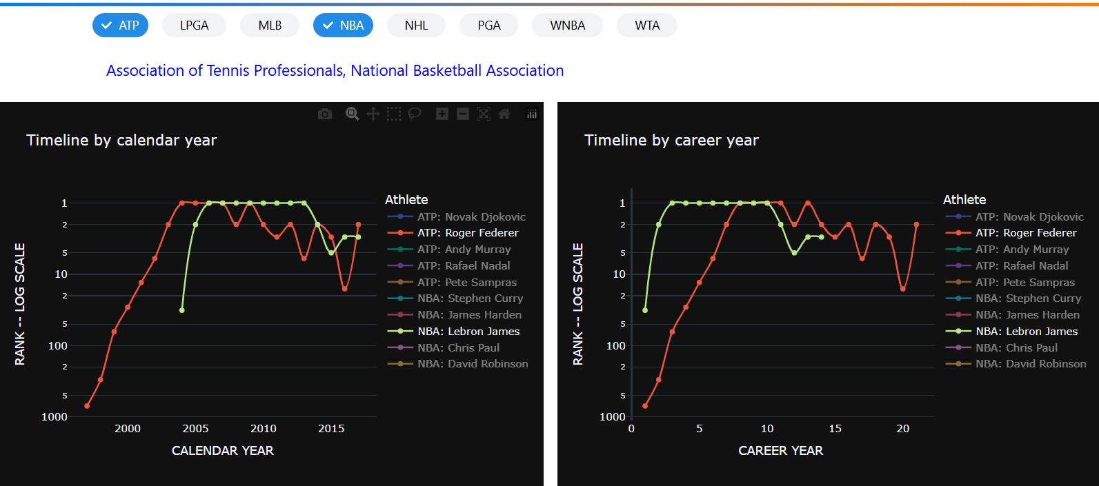
                        "This interactive dashboard visualizes data from The Pudding's article 'One-Hit Wonders in Sports'. "
                        "It analyzes the top 20 players from 8 sports leagues over the last 30 years, exploring the relationship "
                        "between peak performance and career consistency."
                    ], className="lead text-center mx-auto mb-4", 
                       style={**custom_styles['subtitle'], 'max-width': '900px'}),
                    html.Hr(style={'border': '2px solid #667eea', 'width': '100px', 'margin': '0 auto'})
                ], className="text-center")
            ])
        ], className="mb-5"),
        
        # Control Panel
        dbc.Row([
            dbc.Col([
                dbc.Card([
                    dbc.CardHeader([
                        html.I(className="fas fa-sliders-h me-2"),
                        "Control Panel"
                    ], style=custom_styles['control_header']),
                    dbc.CardBody([
                        dbc.Row([
                            dbc.Col([
                                html.Label([
                                    html.I(className="fas fa-trophy me-2"),
                                    "Select League:"
                                ], className="fw-bold mb-2", style={'color': '#495057'}),
                                dcc.Dropdown(
                                    id='league-dropdown',
                                    options=[{'label': i.upper(), 'value': i} for i in athlete_stats['league'].unique()],
                                    value='nba',
                                    multi=False,
                                    placeholder="Select a league...",
                                    className="mb-3",
                                    style={
                                        'border-radius': '10px',
                                        'border': '2px solid #e9ecef'
                                    }
                                )
                            ], md=6),
                            dbc.Col([
                                html.Label([
                                    html.I(className="fas fa-star me-2"),
                                    "Peak Performance (Min):"
                                ], id="performance-label", className="fw-bold mb-2", 
                                       style={'color': '#495057'}),
                                html.Div([
                                    dcc.Slider(
                                        id='performance-threshold-slider',
                                        min=0,
                                        max=1000,
                                        step=10,
                                        value=0,
                                        marks={int(val): {'label': f'{int(val)}', 'style': {'color': '#667eea', 'font-weight': 'bold'}} 
                                              for val in np.linspace(0, 1000, 5)},
                                        className="mb-3"
                                    )
                                ], style=custom_styles['slider_container']),
                                dbc.Tooltip(
                                    "Peak performance is calculated as 1 / (rank + 1) * 1000. A higher score indicates a better performance in a given year.",
                                    target="performance-label",
                                    placement="bottom"
                                )
                            ], md=6)
                        ]),
                        dbc.Row([
                            dbc.Col([
                                html.Label([
                                    html.I(className="fas fa-chart-line me-2"),
                                    "Consistency (Min):"
                                ], id="consistency-label", className="fw-bold mb-2",
                                       style={'color': '#495057'}),
                                html.Div([
                                    dcc.Slider(
                                        id='consistency-threshold-slider',
                                        min=0,
                                        max=1,
                                        step=0.05,
                                        value=0,
                                        marks={round(val, 2): {'label': f'{round(val, 2)}', 'style': {'color': '#667eea', 'font-weight': 'bold'}} 
                                              for val in np.linspace(0, 1, 5)},
                                        className="mb-3"
                                    )
                                ], style=custom_styles['slider_container']),
                                dbc.Tooltip(
                                    "Consistency is the ratio of an athlete's career years that they finished in the top 10.",
                                    target="consistency-label",
                                    placement="bottom"
                                )
                            ], md=6),
                            dbc.Col([
                                html.Label([
                                    html.I(className="fas fa-calendar-alt me-2"),
                                    "Longevity (Min):"
                                ], id="longevity-label", className="fw-bold mb-2",
                                       style={'color': '#495057'}),
                                html.Div([
                                    dcc.Slider(
                                        id='longevity-threshold-slider',
                                        min=0,
                                        max=20,
                                        step=1,
                                        value=0,
                                        marks={int(val): {'label': f'{int(val)}', 'style': {'color': '#667eea', 'font-weight': 'bold'}} 
                                               for val in np.linspace(0, 20, 5)},
                                        className="mb-3"
                                    )
                                ], style=custom_styles['slider_container']),
                                dbc.Tooltip(
                                    "Longevity is the total number of career years for the athlete documented in the data.",
                                    target="longevity-label",
                                    placement="bottom"
                                )
                            ], md=6)
                        ]),
                        # Radio items with better styling
                        dbc.Row([
                            dbc.Col([
                                html.Div([
                                    html.Label([
                                        html.I(className="fas fa-chart-bar me-2"),
                                        "Select Chart:"
                                    ], className="fw-bold mb-3", style={'color': '#495057'}),
                                    dcc.RadioItems(
                                        id='graph-selector-radio',
                                        options=[
                                            {'label': [
                                                html.I(className="fas fa-star me-2"),
                                                'Career Trajectory: Peak vs. Consistency'
                                            ], 'value': 'constellation'},
                                            {'label': [
                                                html.I(className="fas fa-line-chart me-2"),
                                                'Evolution of Annual Performance Score'
                                            ], 'value': 'performance_year'},
                                            {'label': [
                                                html.I(className="fas fa-trophy me-2"),
                                                'Evolution of Top 10 Ranking'
                                            ], 'value': 'consistency_year'}
                                        ],
                                        value='constellation',
                                        className="d-flex flex-wrap justify-content-center",
                                        inputClassName="form-check-input me-2",
                                        labelClassName="form-check-label me-3 mb-2 p-2 rounded",
                                        style={'font-weight': '500'}
                                    )
                                ], style=custom_styles['radio_container'])
                            ])
                        ]),
                    ])
                ], style=custom_styles['control_card'])
            ])
        ], className="mb-4"),
        
        # Main content with graphs and stats
        dbc.Row([
            # Column for all graphs (9/12 of the row)
            dbc.Col([
                dbc.Card([
                    dbc.CardHeader([
                        html.I(className="fas fa-chart-area me-2"),
                        "Performance Analysis"
                    ], style=custom_styles['control_header']),
                    dbc.CardBody([
                        # Main constellation graph container
                        html.Div(id='main-graph-container', children=[
                            dcc.Graph(id='main-graph', style={'height': '600px'}, 
                                     config={'displayModeBar': True, 'displaylogo': False}),
                        ]),
                        # Performance by year graph container (initially hidden)
                        html.Div(id='performance-graph-container', style={'display': 'none'}, children=[
                            html.H5([
                                html.I(className="fas fa-chart-line me-2"),
                                "Evolution of Annual Performance Score"
                            ], className="text-center mt-3 mb-4", style={'color': '#495057'}),
                            dcc.Graph(id='performance-by-year-graph', style={'height': '600px'},
                                     config={'displayModeBar': True, 'displaylogo': False}),
                        ]),
                        # Consistency by year graph container (initially hidden)
                        html.Div(id='consistency-graph-container', style={'display': 'none'}, children=[
                            html.H5([
                                html.I(className="fas fa-trophy me-2"),
                                "Evolution of Top 10 Ranking"
                            ], className="text-center mt-3 mb-4", style={'color': '#495057'}),
                            dcc.Graph(id='consistency-by-year-graph', style={'height': '600px'},
                                     config={'displayModeBar': True, 'displaylogo': False}),
                        ])
                    ])
                ], style=custom_styles['graph_card'])
            ], md=9),

            # Column for athlete details and stats cards (3/12 of the row)
            dbc.Col([
                dbc.Button([
                    html.I(className="fas fa-redo me-2"),
                    "Reset Selection"
                ], id="reset-button", className="w-100 mb-3",
                   style=custom_styles['reset_button']),
                dbc.Card([
                    dbc.CardHeader([
                        html.I(className="fas fa-user-astronaut me-2"),
                        "Athlete Details"
                    ], style=custom_styles['control_header']),
                    dbc.CardBody([
                        html.Div(id='star-details', className="mb-3")
                    ], style={'min-height': '200px'})
                ], style=custom_styles['details_card']),
            ], md=3)
        ], className="mb-4"),
        
        # Footer
        dbc.Row([
            dbc.Col([
                html.Hr(className="my-4", style={'border': '1px solid #dee2e6'}),
                html.P([
                    html.I(className="fas fa-code me-2"),
                    "Dashboard developed with Python | Plotly | Dash. Data courtesy of ",
                    html.A("The Pudding", href="#", className="text-decoration-none", 
                           style={'color': '#667eea', 'font-weight': '500'}),
                    "."
                ], className="text-center mb-0", style=custom_styles['footer'])
            ])
        ])
    ], style=custom_styles['content_wrapper'])
], style=custom_styles['main_container'])

])

New Callback to control which graph is visible

@app.callback(
[Output(‘main-graph-container’, ‘style’),
Output(‘performance-graph-container’, ‘style’),
Output(‘consistency-graph-container’, ‘style’)],
[Input(‘graph-selector-radio’, ‘value’)]
)
def update_graph_visibility(selected_graph):
if selected_graph == ‘constellation’:
return {‘display’: ‘block’}, {‘display’: ‘none’}, {‘display’: ‘none’}
elif selected_graph == ‘performance_year’:
return {‘display’: ‘none’}, {‘display’: ‘block’}, {‘display’: ‘none’}
elif selected_graph == ‘consistency_year’:
return {‘display’: ‘none’}, {‘display’: ‘none’}, {‘display’: ‘block’}
return {‘display’: ‘block’}, {‘display’: ‘none’}, {‘display’: ‘none’} # Fallback

Callback to manage the selection of up to 3 athletes

@app.callback(
Output(‘selected-athletes-store’, ‘data’),
Input(‘main-graph’, ‘clickData’),
State(‘selected-athletes-store’, ‘data’)
)
def update_selected_athletes_list(click_data, current_selection):
if not click_data:
return dash.no_update

clicked_name = click_data['points'][0]['customdata'][0]

if clicked_name in current_selection:
    current_selection.remove(clicked_name)
elif len(current_selection) < 3:
    current_selection.append(clicked_name)

return current_selection

Callback for the reset button

@app.callback(
Output(‘selected-athletes-store’, ‘data’, allow_duplicate=True),
Input(‘reset-button’, ‘n_clicks’),
prevent_initial_call=True
)
def reset_selection(n_clicks):
if n_clicks:
return
return dash.no_update

Callback to update the main constellation graph and the statistics

@app.callback(
[Output(‘main-graph’, ‘figure’)],
[Input(‘league-dropdown’, ‘value’),
Input(‘performance-threshold-slider’, ‘value’),
Input(‘consistency-threshold-slider’, ‘value’),
Input(‘longevity-threshold-slider’, ‘value’),
Input(‘selected-athletes-store’, ‘data’)]
)
def update_constellation_and_stats(selected_league, perf_threshold, consist_threshold, longevity_threshold, selected_athletes):
# Filter data based on selected leagues and the new threshold sliders
filtered_df = athlete_stats[
(athlete_stats[‘league’] == selected_league) &
(athlete_stats[‘peak_performance’] >= perf_threshold) &
(athlete_stats[‘consistency’] >= consist_threshold) &
(athlete_stats[‘career_years’] >= longevity_threshold)
].copy()

fig = go.Figure()

if filtered_df.empty:
    fig.add_annotation(text="No athletes meet these criteria.",
                           xref="paper", yref="paper", x=0.5, y=0.5,
                           showarrow=False, font=dict(size=16, color="#6c757d"))
else:
    fig = px.scatter(
        filtered_df,
        x='consistency',
        y='peak_performance',
        size='career_years',
        hover_data=['name', 'sport_name', 'league', 'best_rank', 'career_years', 'consistency', 'peak_performance'],
        custom_data=['name'],
        title=f"Career Trajectory: Peak Performance vs. Consistency ({selected_league.upper()})",
        color_discrete_sequence=['#667eea'],
        labels={
            'consistency': 'Consistency →',
            'peak_performance': 'Peak Performance ↑'
        }
    )
    fig.update_traces(
        marker=dict(line=dict(width=2, color='rgba(255,255,255,0.8)')),
        opacity=0.8
    )
    selected_stars_df = filtered_df[filtered_df['name'].isin(selected_athletes)]
    if not selected_stars_df.empty:
        for _, row in selected_stars_df.iterrows():
            fig.add_trace(go.Scatter(
                x=[row['consistency']],
                y=[row['peak_performance']],
                mode='markers',
                marker=dict(
                    size=row['career_years'] * 1.5,
                    color='rgba(255, 215, 0, 0.9)',
                    line=dict(width=3, color='#ff6b6b'),
                    symbol='star'
                ),
                name=f"Selected: {row['name']}",
                showlegend=False
            ))

fig.update_layout(
    template='plotly_white',
    title_font_size=18,
    title_font_color='#495057',
    height=600,
    showlegend=False,
    plot_bgcolor='rgba(0,0,0,0)',
    paper_bgcolor='rgba(0,0,0,0)',
    font=dict(family="Inter, sans-serif")
)

return (fig,)

Callback to update the two new line graphs

@app.callback(
[Output(‘performance-by-year-graph’, ‘figure’),
Output(‘consistency-by-year-graph’, ‘figure’),
Output(‘star-details’, ‘children’)],
[Input(‘selected-athletes-store’, ‘data’)]
)
def update_line_graphs_and_details(selected_athletes):
# Initialize empty figures with annotations
fig_perf = go.Figure()
fig_rank = go.Figure()
star_details =

if not selected_athletes:
    fig_perf.add_annotation(text="Click on athletes in the scatter plot to view their performance trajectory",
                            xref="paper", yref="paper", x=0.5, y=0.5, showarrow=False,
                            font=dict(size=16, color="#6c757d"))
    fig_rank.add_annotation(text="Click on athletes in the scatter plot to view their ranking trajectory",
                               xref="paper", yref="paper", x=0.5, y=0.5, showarrow=False,
                               font=dict(size=16, color="#6c757d"))
    star_details = dbc.Alert([
        html.I(className="fas fa-mouse-pointer fa-2x mb-3 d-block"),
        html.H5("Select Athletes", className="mb-2"),
        html.P("Click on up to 3 athletes in the chart to explore their detailed profiles and performance history.")
    ], color="light", className="text-center border-0", 
       style={'background': 'linear-gradient(135deg, rgba(102, 126, 234, 0.1), rgba(118, 75, 162, 0.1))'})
else:
    history_df = df_clean[df_clean['name'].isin(selected_athletes)].copy()
    
    # Performance by year graph
    fig_perf = px.line(
        history_df, 
        x='year', 
        y='performance_score', 
        color='name',
        labels={
            'year': 'Year',
            'performance_score': 'Performance Score'
        }
    )
    fig_perf.update_layout(
        legend_title_text='Athletes',
        font=dict(family="Inter, sans-serif")
    )
    
    # Evolution of ranking with scatter plot
    top10_history_df = history_df[history_df['rank'] <= 10]
    
    if top10_history_df.empty:
        fig_rank.add_annotation(text="No years in the top 10 for these athletes.",
                               xref="paper", yref="paper", x=0.5, y=0.5, showarrow=False,
                               font=dict(size=16, color="#6c757d"))
    else:
        fig_rank = go.Figure()
        colors = ['#667eea', '#764ba2', '#ff6b6b']  # Color palette for athletes
        for i, name in enumerate(top10_history_df['name'].unique()):
            athlete_data = top10_history_df[top10_history_df['name'] == name]
            fig_rank.add_trace(go.Scatter(
                x=athlete_data['year'],
                y=athlete_data['rank'],
                mode='lines+markers+text',
                name=name,
                text=athlete_data['rank'],
                textposition="bottom center",
                marker=dict(size=12, symbol='circle'),
                line=dict(width=3, color=colors[i % len(colors)])
            ))

        fig_rank.update_layout(
            title="Evolution of Top 10 Ranking",
            xaxis_title="Year",
            yaxis_title="Ranking",
            yaxis=dict(autorange='reversed', dtick=1),
            template='plotly_white',
            height=600,
            legend_title_text='Athletes',
            font=dict(family="Inter, sans-serif")
        )
    
    # Update star details with enhanced styling
    selected_athlete_df = athlete_stats[athlete_stats['name'].isin(selected_athletes)].copy()
    colors = ['primary', 'success', 'warning']
    
    for i, (_, row) in enumerate(selected_athlete_df.iterrows()):
        star_details.append(
            dbc.Alert([
                html.Div([
                    html.H5([
                        html.I(className="fas fa-user-circle me-2"),
                        f"{row['name']}"
                    ], className="mb-3", style={'color': '#495057'}),
                    html.Div([
                        html.P([
                            html.I(className="fas fa-trophy me-2"),
                            html.Strong("League: "), f"{row['league'].upper()}"
                        ], className="mb-2"),
                        html.P([
                            html.I(className="fas fa-running me-2"),
                            html.Strong("Sport: "), f"{row['sport_name'].title()}"
                        ], className="mb-2"),
                        html.P([
                            html.I(className="fas fa-medal me-2"),
                            html.Strong("Best Rank: "), f"#{int(row['best_rank'])}"
                        ], className="mb-2"),
                        html.P([
                            html.I(className="fas fa-calendar me-2"),
                            html.Strong("Career Years: "), f"{int(row['career_years'])}"
                        ], className="mb-2"),
                        html.P([
                            html.I(className="fas fa-chart-line me-2"),
                            html.Strong("Peak Score: "), f"{row['peak_performance']:.1f}"
                        ], className="mb-2"),
                        html.P([
                            html.I(className="fas fa-star me-2"),
                            html.Strong("Consistency: "), f"{row['consistency']:.2f}"
                        ], className="mb-0")
                    ])
                ])
            ], color=colors[i % len(colors)], className="mb-3", 
               style={'border': 'none', 'border-radius': '10px', 'box-shadow': '0 4px 15px rgba(0,0,0,0.1)'})
        )

fig_perf.update_layout(
    template='plotly_white', 
    height=600, 
    title_font_size=16,
    plot_bgcolor='rgba(0,0,0,0)',
    paper_bgcolor='rgba(0,0,0,0)',
    font=dict(family="Inter, sans-serif")
)
fig_rank.update_layout(
    plot_bgcolor='rgba(0,0,0,0)',
    paper_bgcolor='rgba(0,0,0,0)'
)

return (fig_perf, fig_rank, star_details)

Callback to update the two new line graphs

@app.callback(
[Output(‘performance-threshold-slider’, ‘max’),
Output(‘consistency-threshold-slider’, ‘max’),
Output(‘longevity-threshold-slider’, ‘max’),
Output(‘performance-threshold-slider’, ‘value’),
Output(‘consistency-threshold-slider’, ‘value’),
Output(‘longevity-threshold-slider’, ‘value’)],
[Input(‘league-dropdown’, ‘value’)]
)
def update_slider_properties_on_league_change(selected_league):
league_data = athlete_stats[athlete_stats[‘league’] == selected_league]
perf_max = league_data[‘peak_performance’].max()
consist_max = league_data[‘consistency’].max()
longevity_max = league_data[‘career_years’].max()
return perf_max, consist_max, longevity_max, 0, 0, 0

server = app.server

Elite Athlete Career Trajectory

[adamschroeder]

That’s a smart move, @Mike_Purtell , converting the y-axis to log scale. Makes it a lot easier to read the line chart.
Looking at the timeline by career year (Tennis), it’s interesting to see how the biggest jumps in ranking tend to happen between year 3-5 of an athlete’s career. It’s also amazing to see how Roger Federer was ranked number 2 in the 21st year of his career.

[adamschroeder]

@Avacsiglo21 I’m getting an error page when trying to load your app. Is it working for you?

[Avacsiglo21]

Weird, yes is giving me an erroe it was working, the ohers two apps there are working

[Avacsiglo21]

It´s working again,

[Mike_Purtell]

Thank you @adamschroeder . I had not looked closely at the men’s tennis list, but now that you mention it Roger Federer has an amazing career arc. Here is a screen shot comparing Roger Federer and Lebron James. Both men reached and held the very top rank of their sports for multiple years. Notice how Lebron rose so quickly to #1 and consider that he went straight from high school into the NBA.

[adamschroeder]

And around year 10 of their career they both started dropping, which seems pretty reasonable in such demanding sports. It’s hard for the body to keep up.

[Ester]

One-Hit Wonders – Interactive Sports Timeline Dashboard

The dashboard provides a detailed, interactive visualization of sports data, structured into several key components:

• Key Metrics Overview: The top section highlights primary figures such as total games played, the number of unique players, average games per player, and the top year for games played.
• Sport and League Filters: Users can filter the data by selecting specific sports (e.g., baseball, basketball, golf, hockey, tennis) and leagues, or adjust the view based on selected years.
• Stacked Timeline Chart: A visual, stacked bar chart illustrates the total games played each year, broken down by sport, helping users spot trends and peaks over time.
• Games Played vs. Rank Scatter Plot: This chart visualizes the relationship between player rank and the number of games played across different sports, enabling comparison and analysis of performance distribution.
• Interactive Controls: Various dropdowns and selection boxes make it easy to customize the displayed data according to user interest.

Here is my dashboard on pycafe:

PyCafe - Dash - Dash Color Selector Demo

[Mike_Purtell]

Thanks @adamschroeder. Time catches up with everyone, even Lebron James and Roger Federer. Thats why I decided not to join the NBA or play professional tennis. Not being athletic also had something to do with that choice.

The logarithmic axis is so easy to implement (log_y=True in the px.line block) and renders extremely well in plotly graphs. Happy to work on this data set where using a log axis makes sense.

[Mike_Purtell]

hi @Ester your dashboard in progress looks like progressing very well. Can’t wait to see its final version.

[adamschroeder]

me too, @Mike_Purtell . I always knew I was NBA material but I decided to not do that to my body, plus I didn’t want all that fame

[marieanne]

I concentrated on ATP year-end top3 players 1992 - 2024

Some players were missing, important ones like Andre Agassi. I added them. I saw a comment about the length of a career, today I added the data until 2024, some important careers were only ended recently. I did not do the tennis women because I collected some extra data and for the women, more different players, too much work. AI was a help but less than I sometimes thought.

One remark: this is the year-end ranking, this means that a player like Marcelo Rios reached the top in march 1998, stayed there a few weeks and had his ranking drop. Rankings are decided based on the results of the last 52 weeks. This explains a dot on the rank 2 for the year end but highest rank in career number one.

To correct the direction of the “spline“ but not too much, players who had a ranking in an “in between“ year or start-end career have the line navigate to ranking 4. I hid that part of the chart with a shape. No idea why the ticklabels on the x-axis are a bit horizontally wrong.

No analytical view, just a fun app. Headshots borrowed from the ATP.

App: PyCafe - Dash - ATP end of year top3, 1992 - 2024

[Mike_Purtell]

Hello @marieanne, nice dashboard. Regarding the x-axis alignment one thing to look at is the xanchor parameter. Looks like it may be set to ‘right’, and if changed to ‘left’ it would move your labels to the right toward where they need to be. Just a guess though, could be something completely different. I have used this many times for annotations, but not for axis labels so not really sure. Hope this helps.

[Avacsiglo21]

Rafa Nadal “king of Clay” AND my favorite Pistol Pete Sampras,kkkk. Cool Dashboard Marianne

[marieanne]

Added nickname, forgot.

[marieanne]

Fixed, this part of the conversion to a pandas dt, changing 01/01 to 12/31 was the culprit,

+ pd.offsets.YearEnd()

[adamschroeder]

What a beautiful app, @marieanne . How did you get the images of each player? Was this all AI made?

[marieanne]

Thank you @adamschroeder. The headshots are from the atp tour website, upper right corner. Probably remove them on saturday due to ©. I asked AI for funfacts + careersummary + headshot , in the end there was a lot in the scraping result I didn’t like or was incorrect.